Designing Data-Intensive Applications: Flashcards for a Book Club

• Reliability The system should continue to work correctly (performing the correct function at the desired level of performance) even in the face of adversity (hardware, software,and humans faults).
• Scalability As the system grows (in data volume,traffic volume,or complexity),there should be reasonable ways of dealing with that growth.
• Maintainability Over time,many different people will work on the system (engineering and operations,both maintaining current behavior and adapting the system to new use cases),and they should all be able to work on it productively.

• Fault - one component of the system deviating from spec.
• Failure - the system as a whole stops providing the required service to the user.
• It’s impossible to lower the probability of a fault to zero; when designing fault-tolerant systems, one needs to prevent faults from causing failures.

• Load parameters describe the current load on the system - with them we can discuss growth. The load parameters change per application. Examples of load parameters include requests per second from a web server, ratio of reads to writes in a DB, number of concurrently active users, hit rates of caches.
• Twitter example: Post tweet: 5K/s avg, 12K/s peak. Home timeline: 300K/s. By describing the load parameters we see that the scaling challenge is due to the fact that each user follows many people and each user is followed by many people.

• Performance metrics are what happens when load increases (see Scalability: What are load parameters? #card [[Designing Data-Intensive Applications]] [[DDIA-C1]] [[DDIA-P1]]). There are two ways to look at performance metrics:
  • What happens when you increase load and keep resources the same
  • How many resources you need to add to keep performance the same if you increase load

• Response time
• Latency (etymology: latent)
  • Latency < Response time
• For web app with multiple backends - measure the slowest one
• Percentiles (p50 == median, p90, p99, p99.9)
  • Amazon stopped at p99.9 (it’s worth fixing at 1 out of 1,000 requests, but not 1 out of 10,000 requests).
  • Important to remember that each page load -> 10s of requests, so p95 usually means a page load (on a complex SPA).

Horizontal and vertical scaling.

• Vertical scaling (scaling up): moving to a more powerful machine
• Horizontal scaling (scaling out): distributing the load across multiple smaller machines: simple when stateless but difficult with stateful data systems

• Operability: make it easy for operations teams to keep the system running smoothly.
• Simplicity: Make it easy for new engineers to understand the system by removing complexity.
• Evolve-ability: Make it easy for engineers to make changes to the system in the future, adapting it for unanticipated use cases as requirements change.

• Relational model: tables and joins.
  • Relational DBs: PostgreSQL,MySQL,MSSQL Server,SQLite.
  • Query language: SQL.
• Document model (NoSQL): standalone documents.
  • Document DBs: MongoDB,RethinkDB,CouchDB,DynamoDB.
  • Query language: differs by DB. For Mongo,mongo aggregation pipeline (JSON-like query). Also MapReduce (for distributed queries, see Chapter 10. Batch Processing).
• Graph model (NoSQL): vertices and edges.
  • Graph DBs: Neo4j,Datomic,Titan,Tinkerpop (AWS -> Neptune).
  • Query languages: Gremlin,Neo4j: Cypher,SPARQL,Datomic: Datalog.

• Normalization: the process of organizing a database to reduce redundancy and improve data integrity. Normalization usually involves dividing a database into two or more tables and defining relationships between the tables, which requires many-to-one relationships and don’t fit well with the Document model.
• Denormalization: the process of trying to improve the read performance of a database at the expense of losing some write performance, by adding redundant copies of data or by grouping data. Denormalization is a common practice in the Document model, where joins are not supported.

• Data always has schema - otherwise the app can’t use it. In DBs that do enforce schema explicitly, the schema is enforced on-write. In schema-less DBs the schema is enforced on-read.

• Schema-on-write (traditional approach): the schema is defined before data is written to the database. The database ensures all data written complies with the schema.
• Schema-on-read (flexible schema): the schema is defined when the data is read from the database. The database does not enforce a schema.

• Schema-on-write:
  • Pro: better support for enforcing data integrity
  • Con: less flexibility for querying data
• Schema-on-read:
  • Pro: more flexibility for querying data
  • Con: less support for enforcing data integrity

• This is a pretty complicated question without s single, straightforward answer. Generally there are a few considerations that boil down to WHICH QUERIES you want to run. In modern data apps you usually end up with a few data models.

• OLTP-optimized: Online Transaction Processing systems are the user-facing systems. They see many requests but each request usually pertains to just a few rows. The bottleneck here is usually disk time..
• OLAP-optimized: Online Analytics Processing.

• Main read pattern: OLTP: Small number of records per query fetched by key. OLAP: Aggregate over a large number of records.
• Main write pattern: OLTP: Random-access low latency writes (from user inputs). OLAP: Bulk imports (with ETLs),event streams.
• Primarily used by: End user/customer,via web app. OLAP: Internal analysts for decision making.
• What data represents: OLTP: Latest state of the data (current point in time). OLAP: History of events (facts) that happened over time.
• Dataset size: OLTP: Gigabytes to Terabytes. OLAP: Terabytes to Petabytes.

• One wide table for “facts” that’s very big, and includes references to smaller tables using foreign keys.
• e.g.: the date will be an ID in the “facts” table and there will be a date “dimension” which is used when querying, e.g., “Which products were bought on a holiday?”.

• Instead of storing data by rows, store each column in a “file” and all the files sorted in the same way (so item number 27 in a column file is the value in the 27th row). This is useful since usually OLAP doesn’t query with SELECT * but only the columns needed for the filtering and aggregation. This works well with the star schema, see What is the “star” schema for OLAP? #card [[Designing Data-Intensive Applications]] [[DDIA-C3]] [[DDIA-P1]]

• Log structured - only append to files and delete old ones, never update.
• Update in place - overwrite pages. B-trees are an example.

• SSTables (Sorted String Tables) are a file format for storing key-value pairs, sorted by key. SSTables are immutable and append-only, which makes them suitable for storing data on disk.
• LSM-Trees (Log-Structured Merge-Trees) are a data structure that provides a way to store key-value pairs in a disk-based storage engine. It’s optimized for write-heavy workloads and is used in many databases, including Apache Cassandra and Google’s Bigtable.

A B-tree is a self-balancing tree data structure that maintains sorted data and allows searches, sequential access, insertions, and deletions in logarithmic time. The B-tree is a generalization of a binary search tree in that a node can have more than two children. Unlike self-balancing binary search trees, the B-tree is well suited for storage systems that read and write relatively large blocks of data, such as disks.

In the context of PostgreSQL, B-trees are the default index type and are used for various types of queries.

• Programming language specific, like Python’s pickle or Java’s serializable. Generally not a good choice, since you lock into a specific language (harder to integrate later down the line) and they normally have major security flaws and performance issues.
• Textual formats, like JSON, XML, and CSV. These are human readable and widely used but don’t have builtin support for schemas, are inherently inefficient, and are sometimes vague when talking about binary data.
• Binary-schema formats like Avro, Protobuf, and Thrift. These formats outperform the others in performance, size, backward-and-forwards compatibility, but are not human readable and generally slightly harder to work with.

• No schema: no way to specify what fields are required, what their types are, and what the structure of the data is.
• Ambiguity: e.g., CSV doesn’t specify whether a field is a string or a number.
• Inherent inefficiency: JSON and XML are verbose and don’t compress well.
• Using Binary data in textual formats is problematic (need to add another layer of encoding with base64).

• Through a database
• REST/RPC
• Message brokers (MQs)

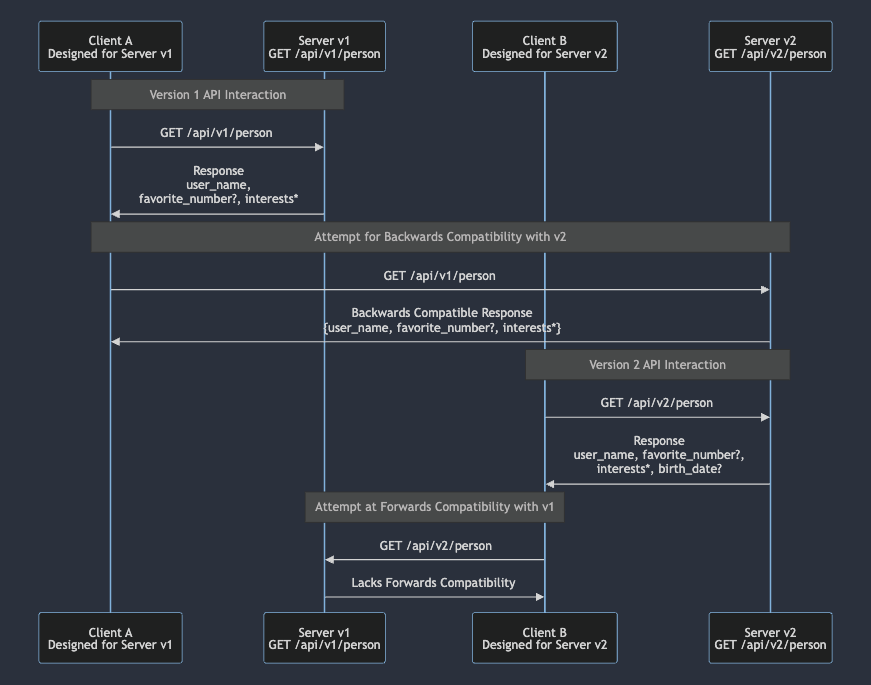
• Forward compatibility: New writer, old reader.
• Backwards compatibility: Old writer, new reader.

Here’s a basic Mermaid diagram that gives an example of this concept.

• Replication: Keep a copy of the same data on several nodes. This provides redundancy.
• Partitioning: Split a big database into smaller subsets called partitions so that different partitions can reside on different nodes (also referred to as sharding).

• Scalability: If data volume, read load, write load grows bigger than a single machine can handle.
• Fault tolerance/high availability: If the app needs to continue working even if a machine/machines/network/data center goes down.
• Latency: Bring the data of an application closer to users geographically.

• Scalability: If data volume, read load, write load grows bigger than a single machine can handle.
• Fault tolerance/high availability: If the app needs to continue working even if a machine/machines/network/data center goes down.
• Latency: Bring the data of an application closer to users geographically.
• Disconnected operation: Allowing an application to continue working when there is a network interruption.

• Single-leader (master-slave) replication: One node is the leader, and the others are followers. The leader receives all the writes and the followers replicate the writes from the leader. The followers can also serve read queries.
• Multi-leader replication: Any node can accept writes. This is more complex than single-leader replication, and it’s hard to resolve conflicts.
• Leaderless replication: All nodes are equal. This is the most complex to implement, but it’s the most fault-tolerant.

Replication can be synchronous or asynchronous. In synchronous replication, the leader waits until followers confirm that they have received the write before reporting success to the user. In asynchronous replication, the leader sends the write to the followers and reports success to the user without waiting for the followers to acknowledge the write.

Async replication can be fast when everything is working well, it can creates an effect called replication lag.

• Read-after-write consistency: If a user writes some data and then reads it back, they should always see the value that they wrote.
• Monotonic reads: After a user has read the value of a key, they should not see the value of that key go backwards in time.
• Consistent prefix reads: Users should see the data in a state that makes sense, for example first the question and only then the answer.

• Each piece of data belongs to exactly one partition.
• The main reason to want partitioning is scalability.

• A large dataset can be distributed across many disks, and the query load can be distributed across many processors.
• When combining replication and partitioning with a leader-follower replication model, each node acts as a leader for some partitions and as a following for other partitions.

• fairness: when the data and query loads are spread evenly,causing n nodes to by able to process $$n$$ times throughput. skew is the opposite. Extreme skew is having ALL data written to and read from a single partition.
• It matters because if you have a lot of skew,you’ll get a partition with load - a hot spot. The the app is data intensive,this will cause a bottleneck.
• Can the DB solve all issues that arise from skew? If you partition by user ID,and there’s one really popular user, the DB can’t compensate for that easily. Today this is an app problem and the app need to redesign the workload (e.g., move all extra-heavy user IDs to their own database, where you partition by user ID + date) and not a DB problem.

• Partition by key range: like encyclopedia volumes.
  • Benefit: Easy range scans.
  • Downside: Certain access patterns can lead to hot spot (e.g. partition by day means the current day gets all the writes, which leaves the rest of the nodes sleepy).}}
• Partition by hash of the key
  • Benefit: data spread randomly and uniformally, no hot spots
  • Downside: data spread randomly :) so no range queries - sort order lost, data spread to all partitions.

• The secondary index is used for searching, it’s usually not unique, and it doesn’t map nearly to partitions. If you partition by user ID, there’s no reason that the name secondary index will map nicely to partitions.

• Partition secondary index by document: each partition maintains its own indexes (local index). This means that you need to do scatter/gather: need to send the query to ALL the partitions, and combine the results. This is prone to tail latency amplification (see Latency (etymology: latent) )
• Partition secondary index by term: indexes are global, and have a different partitioning scheme than the key. The index might point to a document on a different node. This means that updates are async (“eventually consistent”).

• Move data and request from one node to another, because we want to add more CPUs (due to query load), add more disk space (due to dataset size), or remove a failed machine.
• This means shuffling around partitions between nodes.
• What are the three requirements for rebalancing?
  • database needs to stay available for reads and writes
  • after rebalancing we should keep fairness
  • Don’t move data unnecessarily - minimize network and disk I/O load.

• Bad: $$mod ^ n(hash (key))$$ , where $$n$$ = number of nodes. This is bad because when the nodes change, need to move all the data around, which makes rebalancing very expensive.
• Fixed number of partitions: define a LOT more partitions than nodes. When a new node is added,it can copy whole partitions to create fairness. Same for removal. The problem is it’s hard to know how many partitions to add,too many partitions incur overhead but too few make rebalancing costly.
• Dynamic partitioning: When dataset gets to specific size thresholds,split the partition by half. Number of partitions now adepts to the data volume. Pre-splitting is implemented to split load between nodes when the database is just getting started.
• Partition proprotionlly to nodes: dynamic partitioning,but size threshold is impact by node count as well - more nodes,smaller partitions.

• Now that the data is partitioned, when I want to query it, it’s in one out of many partitions. If we have multiple nodes and we support rebalancing, that means the request needs to be routed to the correct node. This is the general problem of “service discovery”.
• At a high level, there are three approaches to this problem:
  • Node level knowledge: I can ask any node - if it knows,it answers,and if it doesn’t it will ask the appropriate node for me. The node a priori knows which key belongs to each node - otherwise,it wouldn’t be able to partition data on write.
    • Examples of this: Cassandra and Riak use a gossip protocol to disseminate any changes in cluster state.
    • Pros: no external service (like ZooKeeper)
    • Cons: more complexity on the nodes themselves.
  • Middleware level knowledge: a middleware that doesn’t handle requests, but just acts as a partition-aware load balancer.
    • Example of this: ZooKeeper - but this might not be true anymore?
  • Client level knowledge: where the client knows about which node to access - be aware of the partitioning and the assignment of partitions to nodes.

• Transactions simplify error scenarios and concurrency issues by executing all reads and writes as one operation.
• They offer safety guarantees, allowing the application to ignore certain potential errors.
• The entire transaction either commits (succeeds) or aborts (fails, with a rollback).

• Atomicity ensures that multiple writes within a transaction are treated as a single operation.
• If a fault occurs after some writes are processed, the transaction can be aborted, not affecting the database’s consistency.
• The term abortability might better describe this property than atomicity.

• Consistency ensures that invariants or rules about the data are always true, maintaining the integrity of the database.
• It’s a property of the application, depending on the application’s notion of invariants, not the database itself.
• Ensures that after a transaction, the data remains correct and valid according to defined rules.

• Isolation keeps concurrently executing transactions separate from each other.
• It aims for serializability, where each transaction pretends it’s the only one running, yielding results as if transactions ran one after another.
• This property protects against concurrency issues, ensuring transactions do not interfere with each other.

• Dirty Reads: Reading uncommitted data from another transaction. 🙈

• Dirty Writes: Overwriting uncommitted data from another transaction. 💥

• Read skew: A client sees different parts of the database at different points in time. Some cases are known as non-repeatable reads. Usually fixed with MVCC (Multi-Version Concurrency Control). 🔄
• Lost Updates: Two transactions read the same data, modify it, and write it back, but one overwrites the other’s changes. Usually fixed with atomic write operations, explicit locking, or compare-and-set. ❌
• Write skew: Two transactions read overlapping data sets and make decisions based on a view of data that changes before the transaction completes. Usually fixed with serializable isolation or explicit locking. 🔀
• Phantom reads: A transaction reads a set of rows that satisfy a search condition and a subsequent read returns a different set due to another transaction’s insert or delete operation. Usually fixed with serializable isolation or explicit locking. 👻

• Durability ensures that once a transaction has successfully committed, the changes it made are permanent and will not be lost even in the event of a system failure.
• This means data has been written to nonvolatile storage or successfully replicated across nodes, safeguarding against hardware faults or crashes.

• Transactions can be aborted and safely retried if an error occurs, ensuring data integrity.
• In leaderless replication datastores, error recovery is the application’s responsibility.
• The capability to abort transactions allows for safe retries, maintaining the database’s consistency and integrity.

• Weak isolation levels attempt to mitigate concurrency issues but do not protect against all of them.
• Common weak isolation levels include Read Committed and Snapshot Isolation, each with specific guarantees against dirty reads and writes.
• They trade-off between performance and strict consistency, allowing some degree of concurrency anomalies to improve system performance.

• Serializable Isolation is the strongest level of isolation in database transactions.
• It ensures that transactions are executed in a way that the outcome is the same as if they had been executed serially, one after the other.
• This isolation level prevents all possible race conditions, making it appear as though each transaction was the only one accessing the database at any time.

• Snapshot Isolation allows transactions to operate on a consistent snapshot of the database.
• It prevents dirty reads and writes by ensuring transactions only see committed data as of the snapshot time.
• Each transaction works with a version of data that remains consistent throughout the transaction, avoiding issues with concurrent modifications.

• Atomic Write Operations: Use database features like atomic increment operations to avoid the need for read-modify-write cycles.

UPDATE counters SET value = value + 1 WHERE key = 'foo';

• Explicit Locking: Lock objects that will be updated to ensure only one transaction can modify them at a time.

• Compare-and-Set: Utilize conditional updates based on the current value to ensure updates are only applied if the data hasn’t changed since it was last read.

UPDATE wiki_pages SET content = 'new content'
  WHERE id = 1234 AND content = 'old content';

• Two-Phase Locking (2PL) is a mechanism to ensure serializability in transactions.
• It involves a phase where locks are acquired on all required resources without releasing any, followed by a phase where all the locks are released.
• 2PL prevents dirty reads, non-repeatable reads, and phantom reads, but can lead to decreased performance due to locking overhead and potential deadlocks.

• SSI is an advanced isolation level that combines snapshot isolation with mechanisms to detect and resolve serialization conflicts.
• It allows transactions to read from a consistent snapshot while also ensuring that the end result is as if the transactions were executed serially.
• SSI aims to provide serializability without the performance penalties associated with traditional locking mechanisms.

• Fault: A component deviating from its spec.
• Failure: The system as a whole stops providing the required service to the user.
• Partial failure: In the context of distributed systems, a partial failure is when some but not all of the nodes in the system are working correctly. The hard part is that partial failures are non-deterministic.

1. Request lost
2. Request waiting in a queue to be delivered later
3. Remote node may have failed
4. Remote node may have temporarily stopped responding
5. Response has been lost on the network
6. The response has been delayed and will be delivered later

A node’s clock may be out of sync with the other nodes (even if you have set up NTP), may jump forwards and backwards unexpectedly, and it’s hard to rely on it since we don’t have a good measure of the clock’s confidence interval.

Also, a process may pause for a substantial amount of time, be declared dead by the other nodes, and then resume without realizing it was paused.

Reasons for process to pause:

• Garbage collector (stop the world)
• Virtual machine can be suspended
• In laptops execution may be suspended
• Operating system context-switches
• Synchronous disk access
• Swapping to disk (paging)
• Unix process can be stopped (SIGSTOP)

• Time-of-day clocks. Return the current date and time according to some calendar (wall-clock time). If the local clock is toof ar ahead of the NTP server, it may be forcibly reset and appear to jump back to a previous point in time. This makes it is unsuitable for measuring elapsed time.
• Monotonic clocks. System.nanoTime(). They are guaranteed to always move forward. The difference between clock reads can tell you how much time elapsed between two checks. The absolute value of the clock is meaningless. NTP allows the clock rate to be speeded up or slowed down by up to 0.05%, but NTP cannot cause the monotonic clock to jump forward or backward. In a distributed system, using a monotonic clock for measuring elapsed time (eg: timeouts), is usually fine.

No, since there are some scenarios that make it hard to know for sure:

• Node semi-disconnected from the rest of the network (ingress OK, egress dead)
• A long GC pause causes the node to be declared dead

• Leader node for a database partition, to avoid split-brain scenarios.
• Master node for a distributed lock for a particular resource, to prevent concurrent access and potential data corruption.
• Unique username or email address, to avoid conflicts and ensure data integrity.

Linearizability is a guarantee about the behavior of operations in a distributed system. It is a guarantee about the real-time ordering of operations. It is the strongest consistency model.

In an eventually consistent database, if you ask two replicas for the current value of a data item, you might get two different answers. In a linearizable database, there is always one correct answer, and it’s the same no matter which replica you ask.

Serializability: Transactions behave the same as if they had executed some serial order.

Linearizability: Recency guarantee on reads and writes of a register (individual object).

Basically, only where it’s very important.

• Locking
• Leader election
• Uniqueness constraints (similar to a lock)
• Cross-channel timing dependencies

Apache ZooKeeper and etcd are often used for distributed locks and leader election.

(These cases are also relevant for “Consensus” - see next card.)

• Total order: If any two operations happen, you can tell which one happened first.
• Causal order: Two events are ordered if the are causally related. Partial order.

The simplest approach would be to have a single copy of the data, but this would not be able to tolerate faults.

• Single-leader repolication is potentially linearizable. 🤔
• Consensus algorithms is linearizable. ✅
• Multi-leader replication is not linearizable. 🚫
• Leaderless replication is probably not linearizable. 🚫

2PC uses a coordinator (transaction manager). When the application is ready to commit, the coordinator begins phase 1: it sends a prepare request to each of the nodes, asking them whether are able to commit.

• If all participants reply “yes”, the coordinator sends out a commit request in phase 2, and the commit takes place.
• If any of the participants replies “no”, the coordinator sends an abort request to all nodes in phase 2.

• Systems of record, which are source of truth,first write here,this is by definition the winner on discreprency
• and derived data systems which are the result of taking existing data and processing/transforming it. Caches,indexes,matviews are examples.

• Services (online), where the interesting metric is response time
• Batch processing (offline), where the interesting metric is throughput
• Stream processing (near-real-time), where the interesting metric is both - so,lower latency than batch and higher throughput than service.

• Automatic deal with datasets that are larger than memory by spilling to disk
• Disk is used well because of sequential I/O optimization: Mergesort,we saw this in chapter 3,storage and retrival.
• Related example: What is column-oriented storage and why does it make sense for OLAP? #card [[Designing Data-Intensive Applications]] [[DDIA-C3]] [[DDIA-P1]]

• Make each program do one thing well.
• Expect that the output of one program will be the input of another: a uniform interface, usually text files
• Design software for early tryout (immutable input)
• Use tooling over unskilled help
• Separation of logic and wiring (just use stdin and stdout)

• Only run on a single machine! That’s where Hadoop comes in.

• Where unix uses stdin stdout, mapreduce uses reading and writing from files on a distributed filesystem.
• HDFS is based on the share-nothing principle, What is shared-nothing (also known as horizontal) partitioning? [[Designing Data-Intensive Applications]] [[DDIA-C6]] [[DDIA-P2]] #card
• How does it work? daemon running on each machine,central server called NameNode - conceptually,this creates a large filesystem without specialized hardware
• HDFS has scaled well in practice.

1. Read input file and break up into records
2. Mapper: Extract the key and value from each record. For each record may emit zero or more key-value pairs. Stateless.
3. Sort by key: this is implicit in MapReduce; the output from the mappers is sorted by key before being passed to the reducers.
4. Reducer: Takes the key-value pairs produced by the mappers, collect all the values that belong to the same key, and calls a reducer with an iterator over that collection of values.

MapReduce can parallelize a computation across many machines, without having to write code to explicitly handle the parallelism. It also handles fault tolerance and data distribution.

It’s parallelization is based on partitioning. The reduce task takes the files from the mappers and merges them together, preserving the sort order.

Single round of sorting means that you can’t do multiple rounds of MapReduce in a single job. This is a problem for some algorithms, like iterative algorithms (e.g., PageRank, K-means clustering). This is why MapReduce workflows are needed.

To handle dependencies between jobs there are workflow schedules for Hadoop like Oozie, Azkaban, Airflow and Pinball. Various high-level tools for Hadoop such as Pig, Hive, Cascading, Crunch, and FlumeJava also set up workflows of multiple MapReduce stages that are wired up automatically.

When a MapReduce job is given a set of files as input, it reads the entire content of all of those files (like a full table scan). When talking about joining data in MapReduce we mean resolving all associations, because we read the entire content of all of those files.

Good example is correlating user activity with user profile data.

Two mappers - one does activity, one does user database. Partition the mapper output by key. One sort is done, the effect is that all activity and database info for the same ID are adjacent in the reducer input. The reducer can then perform the actual join.

One way to look at this architecture is that we’re bringing related data together in the same place by having mappers “send messages” to the reducers. This is a common pattern in distributed systems.

Large amount of data related to the same key (celeb in a social network). Such disproportionately active database records are called linchpin objects or hot keys. If we collect all the data for a hot key in one reducer, that reducer will have a lot of work to do, and the other reducers will be idle. This is a problem because it makes the job slow.

There are a a few algorithms; skewed join in Pig and Hive, sharded join in Crunch. Basically all of them involve sending the hot keys to multiple reducers, and the differences lie in detection.

Reduce-side:

• Pro: No assumptions and the input data
• Con: Slower, because of the sort, copying, and merging

• Broadcast hash join: small table is broadcast to all mappers, and the join is done in the mapper. This is good for small tables that fits in memory.
• Partitioned hash joins: both tables are partitioned in the same way, and the join is done in the mapper. If the partitioning is done correctly, you can be sure that all the records you might want to join are located in the same numbered partition, and so it is sufficient for each mapper to only read one partition from each of the input datasets. This is good for large tables.

In Hive these are called bucketed map joins.

The output of a batch workflow is often a derived data set, such as an index or a cache. This is used in a service (online) system, where the interesting metric is response time. The batch workflow is used to precompute the derived data set, so that the service can respond to user requests more quickly.

• Search indexes; If you need to perform a full-text search over a fixed set of documents, then a batch workflow can be used to build a search index. If the indexed set of documents changes, the index needs to be rebuilt. It’s possible to build indexes incrementally, but it’s more complex.
• ML systems like recommendation engines and classifiers; The batch workflow can be used to train a machine learning model on a large dataset, and the model can then be used to make predictions in a service.
• Materialized views; If you have a database that is too slow to query directly, you can use a batch workflow to precompute the results of the query and store them in a materialized view. The service can then query the materialized view instead of the original database.

Don’t write it directly to the DB using the client lib from within the reducer, because:

1. Network round-trip for each record means poor performance
2. If all mappers/reducers concurrently write to the same output DB it will get overwhelmed
3. MapReduce is normally a clean “all or nothing” operation. If you write from the reducer you create externally visible side effects.

Instead, write the output to a distributed filesystem like HDFS, and then use a separate process to load the data into the database. This is called extract, transform, load (ETL).

In a workflow there are many jobs - the process of writing out the intermediate state between the jobs to files is called materialization of intermediate state. This is a good practice because it makes it easier to debug and inspect the intermediate state, and it also makes it easier to recover from a failure.

Spark, Flink, and other dataflow engines achieve fault tolerance without emitting ALL intermediate state by recomputing from other data that’s still available (latest previous stage that exists or the input data). That means that MapReduce jobs should be deterministic.

• MapReduce job can only start when ALL the previous ones ended
• Mappers are sometimes very simple and could have been chained to the prev reducer
• Writing to HDFS (replication etc.) might be overkill for temporary data

The input is bounded - i.e., of a known and finite size - so the batch process knows when it has finished reading its input. For example, you can sort the input of a batch job, but you can’t do that for a stream because the very last input record could be the one with the lowest key .

In reality a lot of data is unbounded.

• Called an event.
• It’s a small,self-contained,immutable object containing the details of something that happened at some point in time.
• It’s generated by a producer (also publisher/sender), potentially processed by multiple consumers (also subscribers/recipients).
• In a streaming system, related events are usually grouped together into a topic (also stream).

• What happens if the producers send messages faster than the consumers can process them? Three options:
  • drop messages,buffer messages in a queue (what happens when the queue grows),apply backpressure.
• What happens if nodes crash of go offline temporarily - are any messages lost?
  • Durability may require some combo of writing to disk and/or replication
  • Message loss is sometimes acceptable - depends on the application

• UDP multicast, where low latency is important
• Brokerless messaging libraries such as ZeroMQ
• StatsD and Brubeck use unreliable UDP messaging for collecting metrics
• Webhooks, a callback URL

Downsides:

• Require the application code to be aware of the possibility of message loss
• If a consumer if offline, it may miss messages sent while it was down.

DB optimized for message streams. Data is centralized there. It’s a server where producers and consumers connect as clients.

It’s a way to decouple producers and consumers, and to buffer messages if the consumers are not ready to process them immediately. It also provides durability and fault tolerance, removing the burden from the application code (unlike direct messaging).

Using a message broker makes consumers generally async since the producer doesn’t wait for a consumer to pick up a message.

• small working set is assumed.
• automatically delete messages that have been consumed.
• instead of querying the DB, you subscribe to a topic (with support for subset of the topic).
• message brokers do not support arbitrary queries, but notify clients when new data is available.

• ⚖️ Load balancing: Each message is delivered to one of the consumers. The broker may assign messages to consumers arbitrarily.
• 🪭 Fan-out: Each message is delivered to all of the consumers.

In order to ensure that the message is not lost, message brokers use acknowledgements: a client must explicitly tell the broker when it has finished processing a message so that the broker can remove it from the queue.

Note that the message might have been processed and the ACK got lost in the network - to handle this we use atomic commit protocols, see 2PC card.

A log is simply an append-only sequence of records on disk. The same structure can be used to implement a message broker: a producer sends a message by appending it to the end of the log, and consumer receives messages by reading the log sequentially. If a consumer reaches the end of the log, it waits for a notification that a new message has been appended.

To scale to higher throughput than a single disk can offer, the log can be partitioned. Different partitions can then be hosted on different machines. A topic can then be defined as a group of partitions that all carry messages of the same type.

Within each partition, the broker assigns monotonically increasing sequence number, or offset, to every message.

Apache Kafka, Amazon Kinesis Streams, and Twitter’s DistributedLog, are log-based message brokers that work like this.

which messages have been processed: al messages with an offset less than a consumer current offset have already been processed, and all messages with a greater offset have not yet been seen. This adds opportunity for optimization, like skipping messages that have already been processed, and for batching and pipelining.

The offset is very similar to the log sequence number that is commonly found in single-leader database replication. The message broker behaves like a leader database, and the consumer like a follower.

When a consumer cannot keep up with the rate of messages being produced, the number of messages that have been produced but not yet consumed is called the consumer lag. This is a critical metric for monitoring the health of a stream processing system.

Only the slow consumer is affected.

Keeping two systems in sync. As the same or related data appears in several different places, they need to be kept in sync. If an item is updated in the DB, it needs to be updated in the cache, search index, etc.

If doing a batch process to keep the data in sync is too slow, an alternative is dual writes, but that has SERIOUS problems (race conditions, fault tolerance) that lead to inconsistency.

Ultimately the solution is one source of truth.

CDC is the process of observing all data changes in a database, recording them in a log, and making them available in a stream.

Examples

• Debezium, a CDC system for databases
• Bottled Water, a CDC system for PostgreSQL
• Kafka Connect, a framework for building and running connectors that continuously pull in data from other systems and write it to Kafka.

If you keep all the CDC you can rebuilt from scratch.

Normally this is too much so a snapshot is saved with the relevant offset in the CDC.

Event sourcing is a way of persisting the state of a business entity by storing the history of changes as a log of events. Each event represents a state change at a specific point in time. The current state of the entity is derived by replaying the events.

Commands VS Events: A command is a request to change the state of a system, and an event is a record of a state change. A consumer can reject a command, but it can’t reject an event.

• Can’t keep an immutable log forever, so you need to delete old data.
• For administrative/legal reasons you may need to delete data in spite of immutability (GDPR).

1. You can take the data in the events and write it to the database, cache, search index, or similar storage system, from where it can then be queried by other clients.
2. You can push the events to users in some way, for example by sending email alerts or push notifications, or to a real-time dashboard.
3. You can process one or more input streams to produce one or more output streams.

Processing streams to produce other, derived streams is what an operator job does. The one crucial difference to batch jobs is that a stream never ends.

• Complex event processing:
  • Queries are stored long-term, and events from the input streams continuously flow past them in search of a query that matches an event pattern.
  • Esper, IBM InfoSphere Streams, Apama, TIBCO StreamBase, and SQLstream.
• Stream analytics:
  • Aggregating statistics from the stream, such as counting the number of events in a time window, or calculating the average value of a field over time.
  • Stream analytics sometimes use probabilistic algorithms, such as Bloom Filter for set membership, HyperLogLog for counting distinct items, and Count-Min Sketch for approximate frequency counts.
  • Apache Storm, Spark Streaming, Flink, Kafka Streams.
• Maintaining materialized views:
  • A materialized view is a database object that stores the results of a query. It’s a way to precompute the results of a query and store them in a table.
  • Materialized views are used to speed up queries, because the results of the query are already precomputed.
  • Kafka Streams, Samza, and Flink.
• Search on streams:
  • Need to search for a particular event in a stream based on complex criteria, such as full-text search query.

• There’s a difference between event time and processing time. Confusing them will lead to bad data.
• You need to deal with straggler events that arrive after the window has closed. Broadly, two options:
  • Ignore late events.
  • Update the result of the window when a late event arrives.

1. Event time according to the device that generated the event.
2. Sending time according to the device that sent the event.
3. Receiving time according to the server that received the event.

By subtracting 2 from 3 you can estimate drift.

• Tumbling window: Fixed length. If you have a 1-minute tumbling window, all events between 10:03:00 and 10:03:59 will be grouped in one window, next window would be 10:04:00-10:04:59
• Hopping window: Fixed length, but allows windows to overlap in order to provide some smoothing. If you have a 5-minute window with a hop size of 1 minute, it would contain the events between 10:03:00 and 10:07:59, next window would cover 10:04:00-10:08:59
• Sliding window: Events that occur within some interval of each other. For example, a 5-minute sliding window would cover 10:03:39 and 10:08:12 because they are less than 4 minutes apart.
• Session window: No fixed duration. All events for the same user, the window ends when the user has been inactive for some time (30 minutes). Common in website analytics.

• Stream-stream join (Window join):
  • Two streams are joined based on a common key. The join is performed on the fly as events arrive, within some window. The two streams my in fact be the same stream to find related events within a that one stream.
  • Example: Connecting search queries with clicks on search results.
• Stream-table join (Stream enrichment):
  • A stream is joined with a table. The table is usually a lookup table, and the join is performed on the fly as events arrive.
  • Example: Enriching events with user information from a database.
• Table-table join (Materialized view maintenance):
  • Both input streams are database changelogs. Every change in one side in joined with the latest state of the other side.
  • Example: Tweets sent to feeds of followers, follows sent to feeds.

Break the stream into small blocks and tread each blcok like a miniature batch process. This is how Spark Streaming does it.

Checkpointing is the process of writing the state of the computation to a durable storage system, such as HDFS. If the computation fails, it can be restarted from the last checkpoint.

• Exactly-once processing: Each event is processed exactly once. This is the strongest guarantee, but it’s also the most expensive to implement.
• At-least-once processing: Each event is processed at least once, but possibly multiple times. This is the weakest guarantee, but it’s also the cheapest to implement.